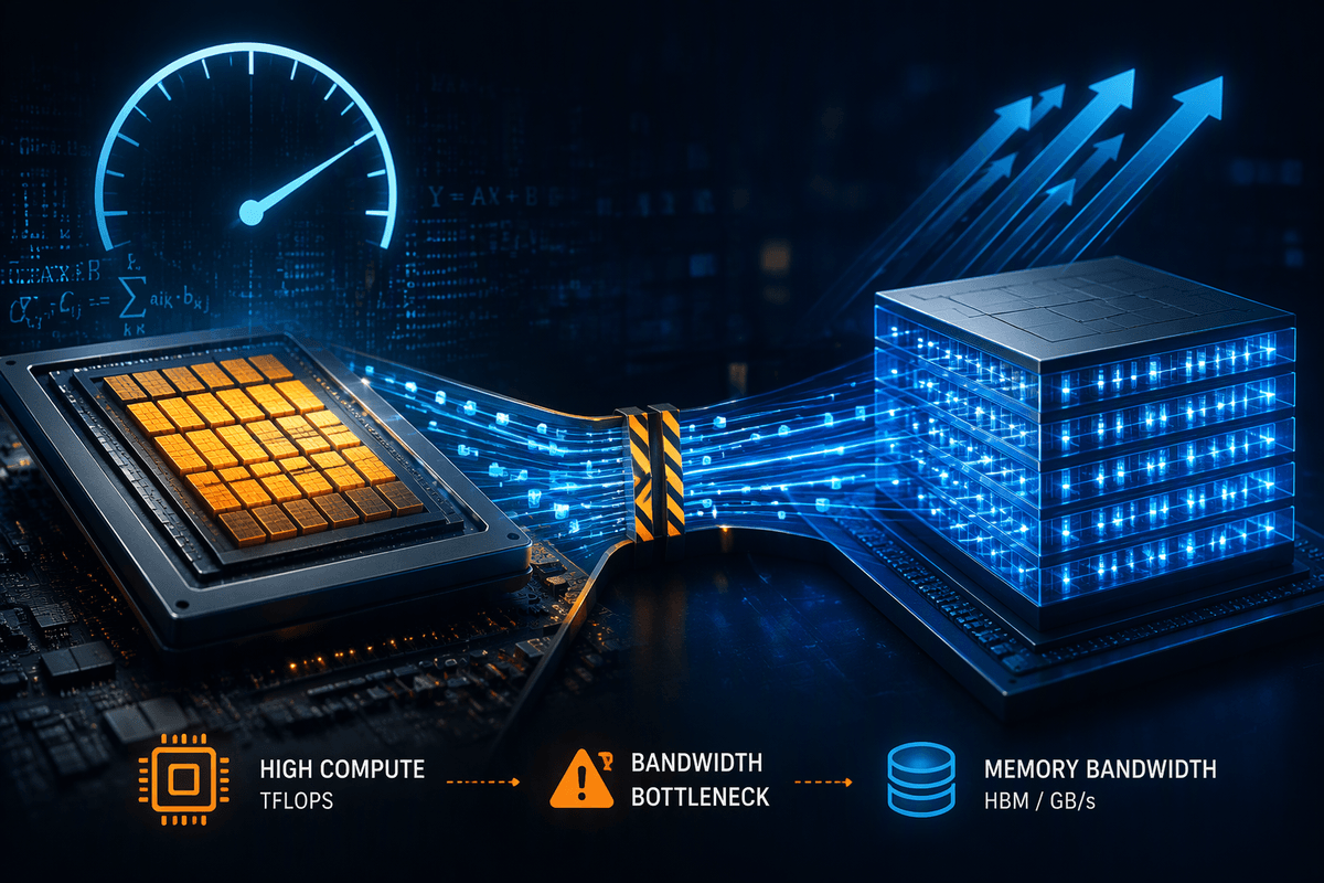
Processing power isn’t the whole AI speed story
You pick a GPU with a huge TFLOPS number, spin up training, and the step time barely improves. Utilization graphs sit low, and you start wondering if the cloud instance is “underpowered” or misconfigured. Often it’s neither. Many AI workloads spend a surprising amount of time moving tensors and weights around rather than multiplying them, so the chip’s compute units wait for data to arrive. Peak compute specs assume a steady stream of operands; real models don’t always provide that stream.
This is why two accelerators with similar TOPS can feel worlds apart once model size, batch size, and memory traffic enter the picture—and why chasing bigger compute can raise cost without raising throughput.
What “memory bandwidth” actually means in practice
Think of memory bandwidth as how fast the processor can pull and push bytes between the compute cores and the accelerator’s “working” memory (typically HBM on modern GPUs). Vendors quote it in GB/s or TB/s, but the practical question is simpler: can the hardware feed your matrix multiplies and attention ops fast enough to keep the cores busy?
In many models, you repeatedly read large weight tensors, activations, and optimizer states, do a modest amount of math on each value, then write results back out. If each byte you load only leads to a small amount of computation (low arithmetic intensity), performance tracks bandwidth more than TFLOPS. Bandwidth is also not the same as latency: you can have high GB/s and still stall on small, irregular accesses. And the headline number is an upper bound—real kernels often see less due to access patterns, data type choices, and contention from concurrent work.
When GPUs wait: the compute–memory imbalance
You can see the compute–memory imbalance in any profiler trace where “the math is ready” but the warps aren’t. A GPU may advertise tens of TFLOPS, yet a single forward pass still has to fetch weights, read activations, and spill intermediates. If those bytes can’t arrive fast enough, the streaming multiprocessors idle and the run looks “slow” even though the compute capacity is untouched. This is why upgrading to a higher-TFLOPS SKU sometimes yields only a small speedup: you bought more engines, but the fuel line stayed the same.
A useful mental model is the roofline: performance is capped by whichever is smaller—compute peak or (bandwidth × arithmetic intensity). Dense GEMMs with large tiles and good reuse push toward compute-bound. Attention, normalization, embedding lookups, small batch inference, and any kernel that rereads big weights with limited reuse tend to be bandwidth-bound. The practical catch is that improving reuse often costs memory (larger batch, checkpointing choices, fused kernels) or engineering time, and sometimes increases latency even if throughput rises.
Training vs inference: two different bandwidth pain points

Training and inference can hit bandwidth limits for different reasons, even on the same model. During training, you aren’t just streaming weights once per layer; you’re also keeping around activations for backprop, reading and writing gradients, and often maintaining extra optimizer state (for example momentum and variance terms). That increases memory traffic and can force more spills to HBM when buffers don’t fit neatly, so step time becomes sensitive to both raw GB/s and how efficiently kernels reuse data. Multi-GPU training adds another bandwidth surface: gradient synchronization can turn interconnect throughput into the limiter even when each GPU looks “underutilized.”
Inference pressure is usually sharper and more uneven. With small batches, you get less reuse of weights per token or request, so you end up repeatedly pulling the same large tensors for relatively little math. Autoregressive decoding makes it worse: each new token can trigger many small reads and writes, where latency and cache behavior matter as much as headline bandwidth. Pushing batch size can improve throughput, but it raises tail latency and may not fit product requirements.
The hidden trips: caches, HBM, and PCIe bottlenecks
You’ll often see a run that looks “bandwidth-bound” even though HBM bandwidth on paper is massive, because the bytes aren’t always coming from HBM in the first place. The fastest path is on-chip: registers and cache. When a kernel has good locality (reusing tiles of weights or activations), those accesses hit cache and the GPU stays busy. When it doesn’t—think embedding tables, scattered attention patterns, or lots of small unfused ops—requests miss cache and spill out to HBM, where high throughput still comes with enough latency to create bubbles. That’s why two GPUs with similar HBM GB/s can behave differently if one has better cache capacity, cache policy, or kernel fusion support.
Then there’s the “hidden trip” off the GPU entirely. If your model weights or KV cache don’t fit, or your pipeline keeps staging tensors on the host, traffic crosses PCIe (or an equivalent host link). Compared with on-package HBM, that link is slow and easy to saturate, and it also burns CPU time in scheduling and copies. Avoiding these trips may mean paying for more VRAM/HBM, using fewer concurrent models per GPU, or investing engineering time to reduce transfers and fuse kernels.
Recognizing bandwidth-bound workloads before you buy hardware
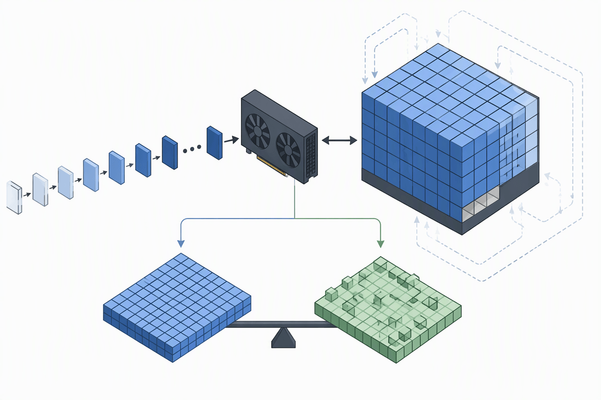
You can usually spot a bandwidth-bound workload without owning the “bigger” GPU yet by looking at a few behaviors. If you switch to a higher-TFLOPS instance and see only a small step-time gain, or if GPU utilization stays low while memory controllers look busy in a profiler, you’re probably limited by data movement. Another tell is sensitivity to batch size: if throughput climbs a lot when you increase batch (more reuse of the same weights per launch), but latency or small-batch performance remains poor, you’re likely paying to reload weights and activations over and over. Models with large embedding tables, attention-heavy blocks, or lots of small kernels also tend to show this pattern.
A rough pre-check is arithmetic intensity: estimate how many bytes you must read/write per token or training step versus how much math you do. If the model’s working set is close to or exceeds device memory, assume extra “hidden trips” and treat the advertised HBM bandwidth as an upper bound you may not reach. Getting these estimates often requires a short profiling run and some back-of-the-envelope accounting, but it’s far cheaper than discovering the bottleneck after a hardware purchase.
Choosing and using hardware with bandwidth in mind
Higher peak TFLOPS won’t improve performance much when kernels are already limited by memory bandwidth. When comparing GPUs or cloud instances, consider memory capacity and bandwidth alongside raw compute power. Check whether the model, optimizer states, or KV cache fit in memory without paging, and compare bandwidth per dollar. Multi-GPU training adds another factor: interconnect speed, since slow links can make synchronization a major source of delay.
Performance also depends on how efficiently workloads use the hardware. Larger batches can improve throughput when latency requirements allow, while mixed precision reduces data movement. Fused attention and normalization kernels help by avoiding unnecessary trips to high-bandwidth memory (HBM). These optimizations require careful testing, as they may reduce memory headroom, increase engineering effort, or affect tail latency in exchange for higher throughput.